Robot Learning Formula Sheet

Fundamentals

Elements of a Reinforcement Learning System

In Reinforcement Learning, an agent interacts with an environment in discrete time steps. At each time step t, the agent receives a state $s_t$ from the environment and selects an action $a_t$ based on its policy $\pi$. The environment then transitions to a new state $s_{t+1}$ and provides a reward $r_{t+1}$ to the agent.

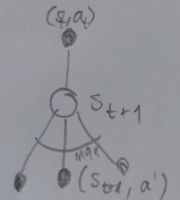
Markov Property

The Markov Property states that the future is independent of the past given the present. In Reinforcement Learning, this means the next state and reward depend only on the current state and action, not on the sequence of events that preceded it.

$$Pr(s_{t+1}=s, r_{t+1}=r \quad | \quad s_0, a_0, r_1 \ldots, r_{t}, s_t, a_t)$$ $$= Pr(s_{t+1}=s, r_{t+1}=r \quad | s_t, a_t)$$

Since the indices in the formula above can be confusing, we can visualize the sequence of states and actions in question like this:

Return

The return at a point t of a trajectory is the sum of the discounted future rewards

$$R_t = r_{\red{t+1}} + \gamma r_{t+2} + \gamma^2 r_{t+3}... = \sum_{i=0}^\infty \gamma^i \cdot r_{t+1+i}$$ $$= r_{t+1} + \gamma R_{t+1}$$

RL Agent goal

The goal of a Reinforcement Learning agent is to find a policy $\pi$ that maximizes the expected return from the start state $s_0$.

$$\mathbb{E}_\pi(R_0)$$

Bellman Equations

The Bellman Equations are fundamental recursive relationships in Reinforcement Learning that relate the value of a state (or state-action pair) to the values of its successor states (or state-action pairs). They are used to compute value functions and are the basis for many RL algorithms.

The Bellman Equation

The Bellman Equation expresses that instead of calculating the discounted cumulative reward by summing up all future rewards, we can decompose it into the immediate reward plus the discounted value of the next state.

State-Value function via Bellman Equation

The value of a state is the average return that can be acquired after that state when following a specific policy:

$$V^\pi(s) = \mathbb{E}_\pi(R_t\quad | \quad s_t=s)$$ $$\mathbb{E}_\pi(r_{t+1} + \gamma V^\pi(s_{t+1})\quad | \quad s_t=s)$$ $$= \sum_a \pi(a|s) \sum_{s'} P_{ss'}^a (R_{ss'}^a + \gamma V^\pi(s'))$$

Action-value function via Bellman Equation

$$Q^\pi(s, a) = \mathbb{E}(R_t\quad | \quad s_t=s, a_t=a)$$ $$= \mathbb{E}_\pi(r_{t+1} + \gamma V^\pi(s_{t+1})\quad |\quad s_t=s, a_t=a)$$ $$= \sum_{s'} P_{ss'}^a (R_{ss'}^a + \gamma V^\pi(s'))$$

Bellman Principle of Optimality

The Bellman principle of optimality states that any part of an optimal policy must itself be optimal for the subproblem starting from that point.

Therefore, the value of a state under an optimal policy, must equal the expected return for the best action from that state. Because subproblems of an optimal solution are themselves optimal: Selecting the next action is a subproblem, so we need to select the optimal action there too.

If a policy is optimal, the remaining decisions must also be optimal

Bellman Optimality Equation For V

$$V^*(s) = \red{\max_a Q^*(s, a)}$$ $$= \max_a \mathbb{E}(r_{t+1} + \gamma V^*(s_{t+1}) \quad|\quad s_t=s, a_t=a)$$ $$= \max_a \sum P_{ss'}^a (R_{ss'}^a + \gamma \red{V^*(s')})$$

Bellman Optimality Equation For Q

$$Q^*(s, a) = \mathbb{E}(r_{t+1} + \gamma \red{\max_{a'} Q^*(s_{t+1}, a')} \quad|\quad s_{t} = s)$$ $$= \sum_{s'} P_{ss'}^a (R_{ss'}^a + \gamma \red{\max_{a'} Q^*(s', a')})$$

Dynamic Programming Methods

Dynamic Programming methods are used to solve Markov Decision Processes (MDPs) when the model of the environment is known. They rely on the Bellman equations to iteratively compute value functions and improve policies.

Iterative Policy Evaluation

Use Bellman Equation for V to iteratively evaluate a policy.

$$V(s_t) = \sum_a \pi(a|s_t) \sum_{s'} P_{s_ts'}^a (R_{s_ts'}^a + \gamma V(s'))$$

Policy Improvement Theorem

If the one-step lookahead using policy $\pi'$ is better than or equal to the value of the current policy $\pi$, $\pi'$ is at least as good as $\pi$.

If for two deterministic policies $\pi$ and $\pi'$ it holds that

$Q^\pi(s, \pi'(s)) \geq V^\pi(s) \quad \forall s$

then $\pi'$ is at least as good as $\pi$.

Policy Iteration

Evaluation step:

$$V(s) = \sum_{s'} P_{ss'}^{\pi(s)} (R_{ss'}^{\pi(s)} + \gamma V(s'))$$

Improvement step:

$$\pi(s) = \text{argmax}_a Q^\pi(s, a) = \text{argmax}_a \sum_{s'} P_{ss'}^a (R_{ss'}^a + \gamma V(s'))$$

Value Iteration

$$V(s) = \max_a Q(s, a) = \max_a \sum_{s'} P_{ss'}^a (R_{ss'}^a + \gamma V(s'))$$

Computing the optimal policy

Given the optimal value function, we can compute the optimal policy.

Optimal Policy given V

Take the action with the highest value for the current state.

$$\pi^*(s) = \text{argmax}_a \sum_{s'} P_{ss'}^a (R_{ss'}^a + \gamma V(s'))$$

Optimal Policy given Q

$$\pi^*(s) = \text{argmax}_a Q(s, a)$$

Temporal Difference Learning

TD($\lambda$) update

$$V(s_t) = V(s_t) + \alpha (R_t^{(\lambda)} - V(s_t))$$

with

$$R_t^{(\lambda)} = (1 - \lambda) \sum_{n=1}^{\infty} \lambda^{(n-1)} R_t^{(n)}$$

where

$$R_t^{(n)} = r_{t+1} + \ldots \gamma^{(n-1)} r_{t+n} + \gamma^n V(s_{t+n})$$

• $(1-\lambda)$ make all terms sum to one
• $\lambda^{n-1}$ weight the returns:
  • $\lambda=0$ only the 1-step return survives: $0^0=1$, $0^n=0$ for all others
  • $\lambda \rightarrow 1$: full episode, monte carlo

Eligibility Traces in backward view

Eligibility traces assign credit to recently visited states. In the backward view, all states are updated with the current TD error, weighted by their eligibility trace.

The eligibility trace decays and is updated like this:

$$e(s) = \gamma \lambda e(s) + 1(s=s_t)$$

In the backward view of TD($\lambda$), the value function is updated for all states:

$$V(s) = V(s) + \alpha e(s) (r_{t+1} + \gamma V(s_{t+1}) - V(s))$$

TD(0) update

When $\lambda=0$, we only consider the one-step return. This is called TD(0) or one-step TD.

$$V(s_t) = V(s_t) + \alpha (r_{t+1} + \gamma V(s_{t+1}) - V(s_t))$$

Monte Carlo Update rule

$$V(s_t) = V(s_t) + \alpha (R_t - V(s_t))$$

For $\alpha=1/n(s)$, where n(s) is the number of times state s has been visited, this is the sample average method (an action-value method mentioned in the beginning of the lecture).

TD Control Methods

Sarsa

Sarsa is a temporal difference learning method that uses action values. We update them using the one-step TD target, so updates can be performed incrementally and not only after the episode is finished.

$$Q(s_t, a_t) = Q(s_t, a_t) + \alpha (r_{t+1} + \gamma Q(s_{t+1}, a_{t+1}) - Q(s_t, a_t))$$

In practice, eligibility traces are used to weigh the influence of the current transition on all past states and decay over time. With them, we can have incremental updates not only to the preceding states but all states.

Sarsa($\lambda$)

Extends SARSA by introducing eligibility traces to speed up learning.

Q-Learning

off-policy, a TD- method that learns Q-values. learns as if we always will choose the optimal action (target policy) but actually still explores with epsilon-greedy (behaviour policy). Might learn an unsafe policy compared to Sarsa.

$$Q(s_t, a_t) = Q(s_t, a_t) + \alpha (r_{t+1} + \gamma \max_{a} Q(s_{t+1}, a) - Q(s_t, a_t))$$

Policy Gradient Methods

REINFORCE

Instead of learning value functions, we directly learn a parameterized policy that selects actions. Use gradient ascent to optimize the policy parameters $\theta$ to maximize the expected return.

$$\nabla_\theta J(\theta) = \mathbb{E}_\pi \left[ \sum_{t=0}^{T-1} \nabla_\theta \log \pi_\theta(s_t, a_t) G_t \right]$$

Example for Policy Gradient Policy

$$\pi_\theta(s) = \text{argmax}_a \hat Q(s,a) = \text{argmax}_a \theta_1 f_1(s,a) + \ldots + \theta_n f_n(s,a)$$

or softmax!

Actor-Critic Methods

REINFORCE has high variance because it uses the full return $G_t$ as an estimate of the action value. Actor-Critic methods reduce this variance by using a learned value function as a baseline.

• The actor represents the policy and is updated via a gradient step, like in REINFORCE.
• The critic represents the value or action value function and provides feedback to the actor, e.g. the td error or advantage estimate. It is updated using TD learning.

Improvements for Policy Gradient Methods

• Introduce a baseline to reduce variance (e.g. the value function)
• Proximal Policy Optimization (PPO): Limit the size of policy updates to ensure stable learning.
  • use the probability ratio between the new policy and the old policy instead of $\nabla_\theta \log \pi$

Linear Methods

LQR

$$s_{t+1} = A_t s_t + B_t a_t$$

LQR reward function

Maximize

$$r(s_0, a_0) + ... + r(s_T, a_T)$$

where

$$r(s_t, a_t) = -(s_t^TQ_ts_t + a_t^TR_ta_t)$$

• $Q_t$ penalize being far from desired state
• $R_t$ penalize large actions

Optimal LQR policy

$$a_t = -L_t s_t = \pi^*(s_t)$$

where

$$L_t = (B_t^T P_{t+1} B_t - R_t)^{-1} B_t^T P_{t+1} A_t$$

Linearizing a function

Given function

$$f(s_t, a_t) = A_t s_t + B_t a_t + w_t$$

We can linearize it with

$$f(s_t, a_t) \approx f(\bar s_t, \bar a_t) + \nabla_s f(\bar s_t, \bar a_t)(s_t - \bar s_t) + \nabla_a f(\bar s_t, \bar a_t)(a_t - \bar a_t)$$

To get back to the $A_t$ and $B_t$ matrices:

$$A_t = \nabla_s f(\bar s_t, \bar a_t)$$ $$B_t = \nabla_a f(\bar s_t, \bar a_t)$$ $$C_t = f(\bar s_t, \bar a_t) - A_t \bar s_t - B_t \bar a_t$$

=> Pull $C_t$ into the state by adding a dimension

Differential Dynamic Programming (DDP)

Similar to LQR, but can handle nonlinear dynamics and non-quadratic cost functions. Linearizes the dynamics and solves the LQR problem iteratively.

Backup Diagrams

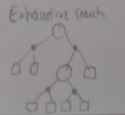
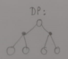
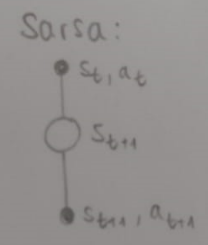
Bellman Equation for V:

Bellman Equation for Q:

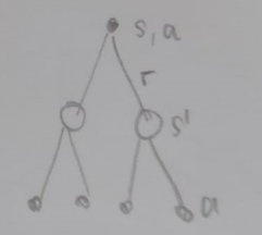
For Bellman Optimality Equation for V:

For Bellman Optimality Equation for Q:

Q-Learning:

Bayesian Methods

Bayesian methods provide a probabilistic framework for modeling uncertainty in Reinforcement Learning. They can be used for model learning, state estimation, and decision-making under uncertainty.

Satz von Bayes

$$P(A|B) = \frac{P(B|A) \cdot P(A)}{P(B)}$$

Or with two states and measurement:

$$p(s_1| z) = \frac{p(z|s_1) \cdot p(s_1)}{p(z)} = \frac{p(z|s_1) \cdot p(s_1)}{p(z|s_1) \cdot p(s_1) + p(z|s_2) \cdot p(s_2)}$$

You can calculate the updated $p(s2)$ after taking an action with the same formula as $p(z)$.

Bayesian Inference

Instead of producing just a single “best estimate” of parameters, Bayesian inference updates probability distributions over them.

Bayesian Model Inference

Bayesian Model Inference can be used to find the model that fits the data the best:

$$\hat M, \hat \theta = \argmax_{M, \theta} p(M, \theta |D_z)$$

It has two steps: Model Fitting and Model Comparison. In Model fitting, we find the parameters that explain the data best for each model. In Model comparison, we choose the model that fits the data best with its optimal parameters.

Fitting:

$$\hat \theta = \argmax_\theta p(\red{\theta| M, D_z})$$

Comparison:

$$\hat M = \argmax_M \int p(M|D_z) = \argmax_M \int p(\red{M, \theta | D_z})\quad d\theta$$

Bayesian Information Criterion BIC

The Bayesian Information Criterion (BIC) is a criterion for model selection among a finite set of models. It is based on the likelihood function and includes a penalty term for the number of parameters in the model.

$$BIC(M) = -2\log(p(\red{D_z |M, \theta})) + k \log n$$

Inverse Reinforcement Learning

In inverse reinforcement learning (IRL), the goal is to infer the underlying reward function that an expert is optimizing, given observations of the expert's behavior.

Feature Expectations

The feature expectations of a policy $\pi$ are the expected discounted sum of feature vectors when following that policy:

$$\mu(\pi) = \mathbb{E} \left[ \sum_{t=0}^\infty \gamma^t \phi(s_t) \right]$$

Max Margin Formula

We try to find weights $W$ so that the reward of the expert policy is better than the reward of any other policy by a margin, using slack variables for expert suboptimality:

$$w^T \mu(\pi_E) \geq w^T \mu(\pi) + m(\pi_E, \pi) - \xi, \quad \forall \pi$$

Apprenticeship Learning

Try to match feature expectations:

$$\mu(\pi) \approx \mu(\pi_E)$$

Does not require the expert to be optimal. Reward ambiguity is not a problem because the feature expectations are matched directly.

Function Approximation

Function approximation is used in Reinforcement Learning to estimate value functions or policies when the state or action space is large or continuous. It allows generalization from seen states to unseen states.

Radial Basis Function Definition

$$\phi_i(s, a) = \exp\left(-\frac{1}{2\sigma^2} \| s - c_i \|^2 \right)$$

Piecewise Linear RBF

$$\phi_i(s, a) = \max\left(0, 1 - \frac{\| s - c_i \|}{b} \right)$$