Quantum Computing Algorithms

In the lecture "Foundations of Quantum Computing", we learned the basic concepts of quantum computing, but we left the actual algorithms for the follow-up course "Quantum Computing Algorithms". The key idea behind many quantum algorithms is the use of phase oracles and amplitude amplification, which I found quite interesting. Below is a summary of these concepts, how they are applied in Grover's algorithm and the Formula Sheet I wrote as exam preparation.

Phase Oracles

For a Boolean function $f: \{0,1\}^n \to \{0,1\}$ , a bit-flip oracle $U_f$ acts as:

U_f |x\rangle |y\rangle = |x\rangle |y \oplus f(x)\rangle

At first glance this does not look very interesting: it writes the output $f(x)$ into the second register by flipping it if $f(x) = 1$ . But here's the trick: if we use $\ket{y} = |-\rangle = \tfrac{1}{\sqrt{2}}(|0\rangle - |1\rangle)$ , it acts as:

U_f |x\rangle |-\rangle = (-1)^{f(x)} |x\rangle |-\rangle

This is a phase oracle. The output $f(x)$ no longer appears on the second qubit, but as a relative phase factor on the first qubit.

This is incredibly useful for quantum algorithms, as it allows us to manipulate the phase of quantum states based on function evaluations.

Why this works: Phase Kickback

The reason why the above works is due to the property of the $|-\rangle$ state. It is called phase kickback.

Remember the polar states are defined as:

|+\rangle = \tfrac{1}{\sqrt{2}} (|0\rangle + |1\rangle), \quad |-\rangle = \tfrac{1}{\sqrt{2}} (|0\rangle - |1\rangle)

They are eigenstates of the Pauli-X operator. It acts on them as follows:

X|+\rangle = +|+\rangle, \quad X|-\rangle = -|-\rangle

This follows a general phenomenon in quantum mechanics: If a qubit is in an eigenstate of an operator, applying that operator only changes the state by a phase factor (the eigenvalue). If a control qubit is in a superposition and the target qubit is in an eigenstate of the operator being controlled, the eigenvalue is transferred back as a relative phase on the control qubit.

This is why using $|-\rangle$ as the auxiliary register in $U_f$ lets us get $(-1)^{f(x)}$ applied to $|x\rangle$ : the eigenvalue from the $X$ operation on $|-\rangle$ has been "kicked back" to the input register.

Grover's Algorithm

Grover’s algorithm is a quantum search method. Imagine searching through $N$ possible items to find one marked item $x^*$ . Classically, we’d need $O(N)$ queries to the function that checks whether $x = x^*$ . Grover’s algorithm reduces this to only $O(\sqrt{N})$ queries by using the phase oracle idea.

In practice, Grover’s algorithm is also useful for SAT problems or any situation where we need to find $x$ such that $f(x) = 1$ .

The idea behind the algorithm is that we can use an oracle to mark the correct solution(s) with a negative phase. If we then reflect all amplitudes about their mean, the marked states will have their amplitudes amplified, while the others are suppressed. Repeating this process a few times will make measuring the correct state very likely. Classically, this would take $O(N)$ queries, but Grover's algorithm can do it in $O(\sqrt{N})$ queries.

Step 1: Uniform superposition

First, we apply Hadamard gates to all qubits to create a uniform superposition:

|s\rangle = H^{\otimes n} |0\rangle^{\otimes n} = \tfrac{1}{\sqrt{2^n}} \sum_{x \in \{0,1\}^n} |x\rangle

This ensures equal amplitude for all possible states.

Step 2: Phase Flip

The oracle then flips the sign of the marked state using a phase oracle, where $x^*$ is the marked item:

S_f = I_{2^n} - 2|x^*\rangle \langle x^*|

This is equivalent to multiplying $\ket{x^*}$ by $-1$ and leaving all other states unchanged.

This may seem silly because to construct $S_f$ we would need to know $x^*$ and would have already solved our problem. In practice, we use a black-box phase oracle that can evaluate $f(x)$ without revealing $x^*$ directly.

Step 3: Diffusion operator

To reflect about the mean, we use the diffusion operator:

D = 2|s\rangle \langle s| - I_{2^n}

We can construct it using Hadamard gates:

D = H^{\otimes n} \big[2|0\rangle^{\otimes n}\langle 0|^{\otimes n} - I_{2^n}\big] H^{\otimes n}

Step 4: Grover iteration

If we put the previous two steps together, we can define the Grover iteration operator:

G = D S_f

Each iteration amplifies the amplitude of $|x^*\rangle$ while suppressing others.

Geometric Viewpoint

It's helpful to see this as a rotation in a 2D subspace: one axis is the marked state $|x^*\rangle$ , the other is the uniform superposition of all unmarked states.

Let $\theta$ be the angle between $|s\rangle$ and $|x^*\rangle$ . Initially, the amplitude of $|x^*\rangle$ in $|s\rangle$ is:

\sin\theta = \frac{1}{\sqrt{2^n}}

The state vector rotates by angle $2\theta$ each iteration. After $r$ iterations, the overlap with the marked subspace is $\sin((2r+1)\theta)$ . Therefore, the success probability is

P(r) = \sin^2\!\left((2r+1)\theta\right)

This oscillates, so it is crucial to choose the right number of iterations.

How many iterations do we need?

From the above formula, we can infer that the probability of measuring $|x^*\rangle$ is maximized when:

r \approx \left\lfloor \tfrac{\pi}{4} \sqrt{\tfrac{2^n}{k}} \right\rfloor

where $k$ is the number of marked solutions.

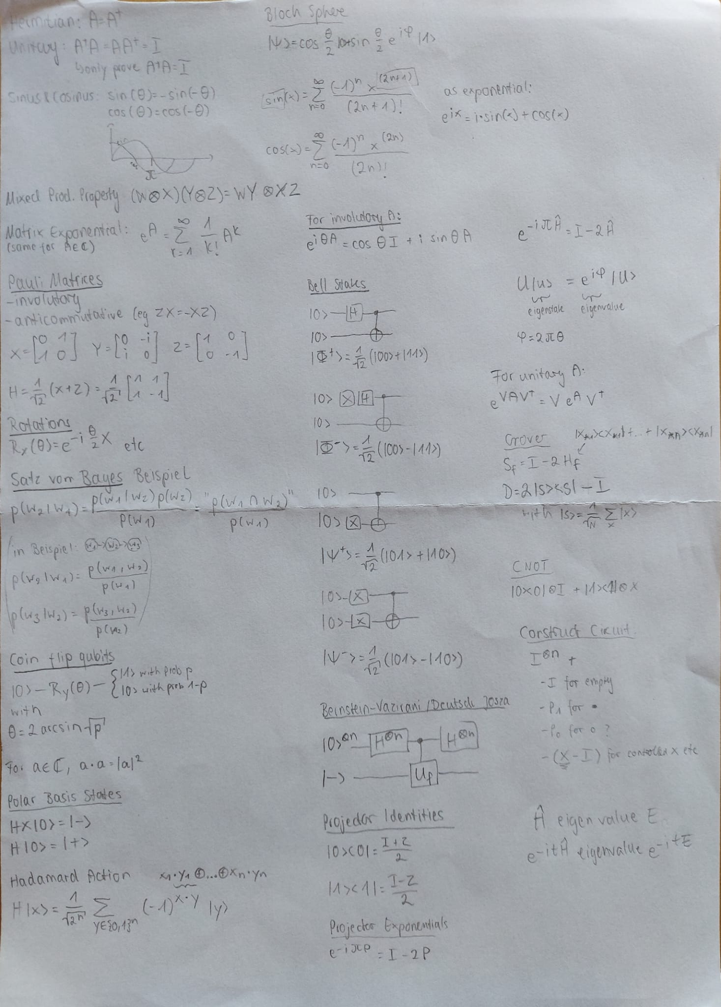
Formula Sheet

Comments

Feel free to leave your opinion or questions in the comment section below.

By clicking on 'Sign in with Github', a login cookie is created. You can undo this at any time by clicking 'Delete Cookie'.