Predicting Bike Rental Demand with Machine Learning
Competition of the ML Club at the University of Bonn
As part of the ML Club at the University of Bonn, we participated in a small competition where the goal was to predict bike rental demand using machine learning.
Task
The dataset provided contained the number of rented bikes per timestamp, as well as additional information such as weather data and holidays. The task was to develop a model that could accurately predict demand on a similar dataset without the actual rental counts. The prediction quality was measured using RMSE (Root Mean Squared Error), which indicates how much the prediction deviates from the actual demand. The challenge was hosted on Kaggle, where participants could upload their predictions for another dataset.
Data Analysis
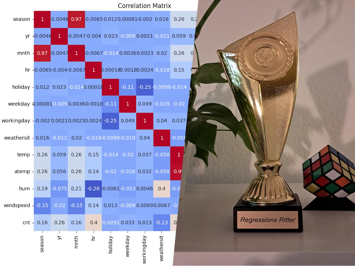
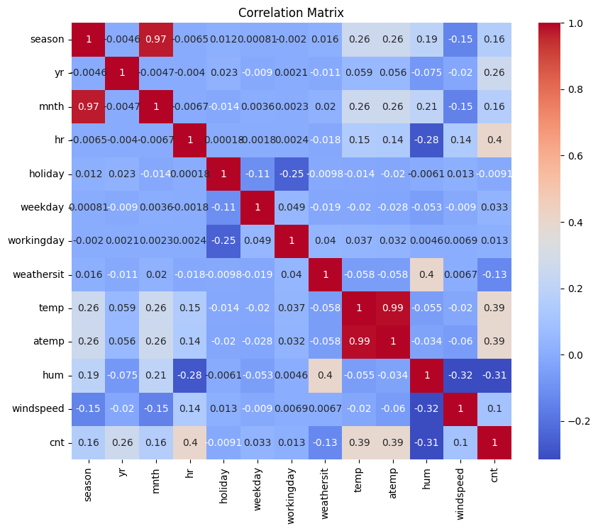
Before developing a model, we examined the data more closely to decide which features to use. A correlation matrix showed that the features temp (temperature) and atemp (feels-like temperature), as well as season (season) and month (month) were strongly correlated. Therefore, we decided not to use the features atemp and season.
Model
To predict demand, we used an XGBoost regression model. First, the data was cleaned by removing outliers in the target variable cntusing the Interquartile Range (IQR) method. Categorical variables were then transformed using one-hot encoding.
The model was trained on the logarithmized target values to smooth the distribution. For hyperparameter optimization, we used RandomizedSearchCVwith 5-fold cross-validation. The most important parameters such as max_depth, learning_rate,subsample, and regularization parameters were searched.
The best model achieved an RMSE of 31.53 and an MAE of 19.24 on the training data. On our own evaluation data, the RMSE was 37.78 and the MAE was 23.27. For comparison: The mean of the target variable cnt is about 190. The result is not bad, but also not outstanding. Since we had limited time, we decided not to further optimize the results and submit the challenge as is.
The most important features, besides the weather data, were especially the hour of the day, the month, and the day of the week.
Code
import xgboost as xgb
import numpy as np
from sklearn.model_selection import RandomizedSearchCV
from sklearn.metrics import mean_squared_error, mean_absolute_error

from os import path
import pandas as pd
from utils import one_hot_all

def load_data():

    file = path.abspath(path.join("data", "train_data_bike.csv"))
    df = pd.read_csv(file)
    df = df.drop(columns=["atemp", "season", "dteday"])
    df = one_hot_all(df)

    print(df.columns.tolist())

    # Use IQR to detect outliers in "cnt"
    Q1 = df["cnt"].quantile(0.25)
    Q3 = df["cnt"].quantile(0.75)
    IQR = Q3 - Q1

    outlier_mask = (df["cnt"] < (Q1 - 1.5 * IQR)) | (df["cnt"] > (Q3 + 1.5 * IQR))
    outliers = df[outlier_mask]
    print(f"Number of outliers: {outliers.shape[0]}")
    outliers[["cnt"]]

    df = df[~outlier_mask].reset_index(drop=True)

    eval_df = df.sample(frac=0.25, random_state=42)
    train_df = df.drop(eval_df.index)
    eval_y = eval_df["cnt"]
    train_y = train_df["cnt"]

    eval_df = eval_df.drop(columns=["cnt"])
    train_df = train_df.drop(columns=["cnt"])
    return train_df, train_y, eval_df, eval_y

train_df, train_y, eval_df, eval_y = load_data()

param_dist = {
    "n_estimators": [2000],
    "max_depth": [5, 6, 7],
    "learning_rate": [0.01, 0.02, 0.03],
    "subsample": [0.4, 0.6, 0.8],
    "colsample_bytree": [0.4, 0.6, 0.8],
    "reg_alpha": [0.6, 0.8, 1],
    "reg_lambda": [1, 5],
    "min_child_weight": [3, 4],
    "gamma": [0, 0.1],
    "max_delta_step": [1, 2, 3],
}

xgb_model = xgb.XGBRegressor(random_state=42, tree_method="hist")
search = RandomizedSearchCV(
    xgb_model,
    param_distributions=param_dist,
    n_iter=40,
    cv=5,
    scoring="neg_root_mean_squared_error",
    n_jobs=-1,
    random_state=42,
)
search.fit(train_df, np.log1p(train_y))  # still train on log-scale
best = search.best_estimator_

y_pred = np.expm1(best.predict(train_df))  # type: ignore
rmse = mean_squared_error(train_y, y_pred) ** 0.5
mae = mean_absolute_error(train_y, y_pred)
print(f"Tuned XGB → RMSE: {rmse:.2f}, MAE: {mae:.2f}")
print(search.best_params_)

y_pred_eval = np.expm1(best.predict(eval_df)) # type: ignore
rmse_eval = mean_squared_error(eval_y, y_pred_eval) ** 0.5
mae_eval  = mean_absolute_error(  eval_y, y_pred_eval)
print(f"Eval → RMSE: {rmse_eval:.2f}, MAE: {mae_eval:.2f}")
Results
Our model achieved an RMSE of 56.897 on the final evaluation data of the challenge, which actually earned us first place.

Comments
Feel free to leave your opinion or questions in the comment section below.