Foundations of Quantum Computing

Recap of the quantum lecture

#Master's Studies#Quantum Computing#University Studies
The module "Foundations of Quantum Computing" covered the basics of quantum mechanics and quantum information theory. I will summarize the most important points below.
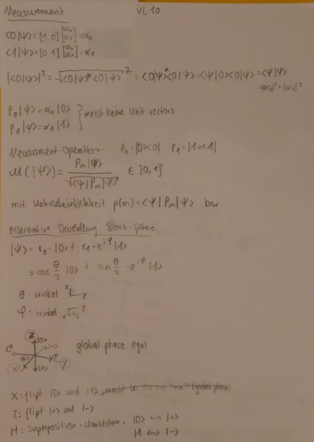
The most important mathematical foundations are summarized in the following cheat sheet:

Cheat Sheet – Mathematical Foundations of Quantum Computing

Standard Qubit States

  • |0⟩ =
(10)\begin{pmatrix} 1 \\ 0 \end{pmatrix}
  • |1⟩ =
(01)\begin{pmatrix} 0 \\ 1 \end{pmatrix}
  • Inner product [a  b](cd)=ac+bd[a \; b] \begin{pmatrix} c \\ d \end{pmatrix} = a \cdot c + b \cdot d

  • Outer product examples:

    • 00=(1000)|0\rangle\langle0| = \begin{pmatrix} 1 & 0 \\ 0 & 0 \end{pmatrix}
    • 01=(0100)|0\rangle\langle1| = \begin{pmatrix} 0 & 1 \\ 0 & 0 \end{pmatrix}
    • 10=(0010)|1\rangle\langle0| = \begin{pmatrix} 0 & 0 \\ 1 & 0 \end{pmatrix}
    • 11=(0001)|1\rangle\langle1| = \begin{pmatrix} 0 & 0 \\ 0 & 1 \end{pmatrix}

Shortcut to calculating outer Products

Note that if you read the ket-bra as a binary number (e.g. 10|1\rangle\langle0| as 2), the binary number corresponds to the index in the matrix where the 1 is. All others are 0.

Shortcut to calculating inner Products

Note that if the 2 numbers in the ket-bra are equal, the inner product returns 1, otherwise 0

  • 00=1\langle 0|0 \rangle = 1
  • 01=0\langle 0|1 \rangle = 0
  • 10=0\langle 1|0 \rangle = 0
  • 11=1\langle 1|1 \rangle = 1

Bra-ket (Inner Products)

Expression Description
10\langle 1\|0 \rangle (01)(10)\begin{pmatrix}0 1 \end{pmatrix} \begin{pmatrix}1 \\ 0 \end{pmatrix}
Bracket bra (horizontal) - ket

Polar Basis States

+=12(0+1)=[1212]|+\rangle = \frac{1}{\sqrt{2}}(|0\rangle + |1\rangle) = \begin{bmatrix} \frac{1}{\sqrt{2}} \\ \frac{1}{\sqrt{2}} \end{bmatrix} =[1212]= \begin{bmatrix} \frac{1}{\sqrt{2}} \\ -\frac{1}{\sqrt{2}} \end{bmatrix}

Pauli Matrices

  • X:
(0110)\begin{pmatrix} 0 & 1 \\ 1 & 0 \end{pmatrix}
  • Y:
(0ii0)\begin{pmatrix} 0 & -i \\ i & 0 \end{pmatrix}
  • Z:
(1001)\begin{pmatrix} 1 & 0 \\ 0 & -1 \end{pmatrix}

Pauli Matrices as outer Products

  • X:
X=01+10=(0110)X = |0\rangle\langle1| + |1\rangle\langle0| = \begin{pmatrix} 0 & 1 \\ 1 & 0 \end{pmatrix}
  • Y:
Y=i01+i10=(0ii0)Y = -i|0\rangle\langle1| + i|1\rangle\langle0| = \begin{pmatrix} 0 & -i \\ i & 0 \end{pmatrix}
  • Z:
Z=0011=(1001)Z = |0\rangle\langle0| - |1\rangle\langle1| = \begin{pmatrix} 1 & 0 \\ 0 & -1 \end{pmatrix}

Hermitian Transpose

For z=a+biz = a + bi, z=abi\quad z^* = a - bi.

Transpose Matrix and complex conjugate its elements:

A=(abcd),A=(acbd) A = \begin{pmatrix} a & b \\ c & d \end{pmatrix}, \quad A^\dag = \begin{pmatrix} a^* & c^* \\ b^* & d^* \end{pmatrix}
  • (Ay)=yA\left( A | y \rangle \right)^\dagger = \langle y | A^\dagger
  • (AB)=BA\left( AB \right)^\dagger = B^\dagger A^\dagger
  • (aA+bB)=aA+bB\left( aA + bB \right)^\dagger = a^* A^\dagger + b^* B^\dagger

Effects on the Basis States

Effects of the Pauli Matrices and the Hadamard gate on the basis states and polar basis states

Gate Effect on |0⟩ Effect on |1⟩ Effect on |+⟩ Effect on |−⟩
X |1⟩ |0⟩ |+⟩ -|-⟩
Y i|1⟩ -i|0⟩ -i|−⟩ i|+⟩
Z +|0⟩ -|1⟩ |-⟩ |+⟩
H |+⟩ |−⟩ |0⟩ |1⟩

Kronecker Product

AB=(a11Ba1nBam1BamnB).A \otimes B = \begin{pmatrix} a_{11}B & \dots & a_{1n}B \\ \vdots & \ddots & \vdots \\ a_{m1}B & \dots & a_{mn}B \end{pmatrix}.
  • Associativity
  • Distributivity
  • Non-commutativity
  • Mixed product property: (WX)(YZ)=(WY)(XZ)(W \otimes X)\,(Y \otimes Z) = (WY) \otimes (XZ)
  • Transpose and complex conjugate distribution: (XY)T=XTYT(X \otimes Y)^T = X^T \otimes Y^T (XY)=XY(X \otimes Y)^* = X^* \otimes Y^*

Hadamard Gate

H1=12(1111)H_1 = \frac{1}{\sqrt{2}} \begin{pmatrix} 1 & 1 \\ 1 & -1 \end{pmatrix}

(For higher dimensions: Hn=H2Hn1H_n = H_2 \otimes H_{n-1}, etc.)

Also,

H=12(X+Z)H = \frac{1}{\sqrt{2}} (X + Z)

and

HXH=ZHXH = Z

Vector Space Axioms

\oplus

  1. Commutativity of addition
  2. Associativity of addition
  3. Neutral element (existence of a zero vector)
  4. Inverse elements (existence of additive inverses)

\otimes

  1. Distributivity (over vector addition and scalar multiplication)
    • a(xy)=axaya \cdot (x \oplus y) = a \cdot x \oplus a \cdot y
    • (a+b)x=axbx(a + b) \cdot x = a \cdot x \oplus b \cdot x
  2. Scalar associativity (compatibility of scalar multiplication)
  3. Unity of scalar multiplication (existence of multiplicative identity)

Key Matrix Definitions

  • Hermitian: A=AA = A^\dagger

    • Hermitian matrices have real diagonal entries.
    • Eigenvalues of a Hermitian matrix are real.
  • Normal: AA=AAAA^\dagger = A^\dagger A

  • Unitary: AA=AA=IA^\dagger A = A A^\dagger = I

    • Eigenvalues have absolute value 1.
    • det(A)\det(A) has absolute value 1.

Useful Facts

  • Trace(AA) = sum of eigenvalues.

  • Det(AA) = product of eigenvalues.

  • Rank(AA) = maximum number of linearly independent rows (or columns).

  • Exponential of a matrix:

eA  =  k=01k!Ake^{A} \;=\; \sum_{k=0}^{\infty} \frac{1}{k!}\,A^k
  • Log of a matrix (for suitably defined AA):
log(A)  =  k=1(1)k+1(AI)kk\log(A) \;=\; \sum_{k=1}^{\infty} (-1)^{k+1} \frac{(A - I)^k}{k}

sin\sin and cos\cos

Series expansions (for scalar xx):

sin(x)=n=0(1)nx2n+1(2n+1)!,cos(x)=n=0(1)nx2n(2n)!\sin(x) = \sum_{n=0}^\infty \frac{(-1)^n x^{2n+1}}{(2n+1)!}, \quad \cos(x) = \sum_{n=0}^\infty \frac{(-1)^n x^{2n}}{(2n)!}

y-intercepts:

sin(0)=0cos(0)=1\sin(0)=0 \quad \cos(0)=1 \quad

Symmetry:

sin(θ)=sin(θ)cos(θ)=cos(θ)\sin(-\theta)=-\sin(\theta) \quad \cos(-\theta)=cos(\theta)

Roots:

sin(πn)=0cos(12π+πn)=0\quad \sin(\pi * n) = 0 \quad \cos(\frac{1}{2}\pi+\pi * n) = 0

Relation to exe^x:

eix=isin(x)+cos(x)e^{ix}=i*\sin(x)+\cos(x)

Idempotent and Projection

  • Idempotent: A2=AA^2 = A.

    • Every idempotent matrix is a projection matrix (and vice versa).
    • Eigenvalues of an idempotent matrix are 0 or 1.
    • tr(A)=rank(A)\text{tr}(A) = \text{rank}(A) if AA is idempotent.
    • If AA and BB are idempotent, then ABAB is idempotent only if AB=BAAB=BA.
    • If AA and BB are idempotent, then A+BA+B is idempotent only if AB=BAAB=-BA.
    • IAI-A idempotent, if A idempotent
  • Projection matrix PP:

    • P=uu(if u=1, projects onto span{u}) P = \lvert u \rangle \langle u \rvert \quad \text{(if $\|u\|=1$, projects onto $\text{span}\{u\}$)}
    • uu=1uu\langle u \mid u \rangle = 1 \Rightarrow \mid u \rangle \langle u \mid is idempotent
    • Satisfies P2=PP^2 = P.

Involutory Matrices

  • Involutory: A2=IA^2 = I.
    • Eigenvalues are ±1\pm 1.
    • det(A)=±1\det(A) = \pm 1.
    • AA is idempotent I+A2\Leftrightarrow \frac{I + A}{2} is idempotent.
    • AA is idempotent IA2\Leftrightarrow \frac{I - A}{2} is idempotent.
    • Powers of AA alternate between II and AA.
    • A,BA, B involutory \Rightarrow A,BA, B only involutory if AB=BAAB=BA

Permutation Matrices

  • Permutation matrix PP:
    • Square, entries in {0,1}\{0,1\}.
    • Exactly one "1" in each row and column, others 0.
    • Sums of each row and each column are 1.
    • Orthogonal, unitary, and invertible.
    • If you multiply a permutation matrix by itself often enough, you eventually get the identity.
    • Product of two permutation matrices is another permutation matrix.

Eigenvectors and Eigenvalues

  • For matrix AA, an eigenvector x\mathbf{x} and eigenvalue λ\lambda satisfy
Ax=λx.A \mathbf{x} = \lambda \mathbf{x}.
  • For a Hermitian AA, λ\lambda is real.
  • For a Hermitian Matrix, its Eigenvectors are orthogonal
  • For a unitary AA, λ=1\lvert \lambda \rvert = 1.
  • For an idempotent AA, λ{0,1}\lambda \in \{0, 1\}.
  • For an involutory AA, λ{±1}\lambda \in \{\pm 1\}.

Permutation Matrices

  • Permutation matrix PP:
    • Square, entries in {0,1}\{0,1\}.
    • Exactly one "1" in each row and column, others 0.
    • Sums of each row and each column are 1.
    • Orthogonal, unitary, and invertible.
    • If you multiply a permutation matrix by itself often enough, you eventually get the identity.
    • Product of two permutation matrices is another permutation matrix.

The mentioned topics are based on concepts of linear algebra, which were assumed to be known. In the following I summarize the concepts learned in previous modules:

More or less relevant linear algebra concepts

Eigenvectors and Eigenvalues

  • For matrix AA, an eigenvector x\mathbf{x} and eigenvalue λ\lambda satisfy
Ax=λx.A \mathbf{x} = \lambda \mathbf{x}.

Determinant of a Matrix

For a 2x2 Matrix

For a 2x2 matrix

A=(abcd),A = \begin{pmatrix} a & b \\ c & d \end{pmatrix},

the determinant is given by:

det(A)=adbc.\det(A) = ad - bc.

Using Cofactor Expansion

For an n×nn \times n matrix, the determinant can be calculated using cofactor expansion along any row or column. For example, expanding along the first row:

det(A)=j=1n(1)1+ja1jdet(A1j),\det(A) = \sum_{j=1}^{n} (-1)^{1+j} a_{1j} \det(A_{1j}),

where A1jA_{1j} is the (n1)×(n1)(n-1) \times (n-1) submatrix obtained by removing the first row and jj-th column of AA.

For example, for a 3x3 matrix

A=(abcdefghi),A = \begin{pmatrix} a & b & c \\ d & e & f \\ g & h & i \end{pmatrix},

the determinant is given by:

det(A)=aefhibdfgi+cdegh.\det(A) = a \begin{vmatrix} e & f \\ h & i \end{vmatrix} - b \begin{vmatrix} d & f \\ g & i \end{vmatrix} + c \begin{vmatrix} d & e \\ g & h \end{vmatrix}.

Properties of Determinants

  • Multiplicative Property: det(AB)=det(A)det(B)\det(AB) = \det(A) \det(B)
  • Transpose: det(AT)=det(A)\det(A^T) = \det(A)
  • Inverse: If AA is invertible, det(A1)=1det(A)\det(A^{-1}) = \frac{1}{\det(A)}
  • Determinant of Identity Matrix: det(I)=1\det(I) = 1
  • Row Operations:
    • Swapping two rows multiplies the determinant by 1-1.
    • Multiplying a row by a scalar kk multiplies the determinant by kk.
    • Adding a multiple of one row to another row does not change the determinant.

Kernel, Image, and Related Concepts

Kernel (Null Space)

The kernel (or null space) of a matrix AA, denoted as ker(A)\ker(A) or null(A)\text{null}(A), is the set of all vectors x\mathbf{x} such that Ax=0A\mathbf{x} = \mathbf{0}. In other words, it is the set of solutions to the homogeneous equation Ax=0A\mathbf{x} = \mathbf{0}.

Image (Column Space)

The image (or column space) of a matrix AA, denoted as im(A)\text{im}(A) or col(A)\text{col}(A), is the set of all vectors that can be expressed as AxA\mathbf{x} for some vector x\mathbf{x}. It is the span of the columns of AA.

Rank

The rank of a matrix AA, denoted as rank(A)\text{rank}(A), is the dimension of the image (column space) of AA. It represents the maximum number of linearly independent columns of AA.

Nullity

The nullity of a matrix AA, denoted as nullity(A)\text{nullity}(A), is the dimension of the kernel (null space) of AA. It represents the number of linearly independent solutions to the homogeneous equation Ax=0A\mathbf{x} = \mathbf{0}.

Rank-Nullity Theorem

The rank-nullity theorem states that for any m×nm \times n matrix AA:

rank(A)+nullity(A)=n,\text{rank}(A) + \text{nullity}(A) = n,

where nn is the number of columns of AA.

What follows are the rest of my notes that I did not have time to add in my Markdown file.MeasurementGatesProgrammableMulti

Worksheets

General Bit Manipulation

  • Calculate required bits for a binary number: log2(n)+1\lfloor\log_2(n)\rfloor+1
  • Convert a decimal number to binary: mod(n,2),div(n,2)\text{mod}(n,2),\text{div}(n,2)
  • Convert a decimal number to binary grey code: base2(n(n>>1))base2(n^{(n>>1)})*
    • Bitshift right by 1: equivalent to dividing by 2

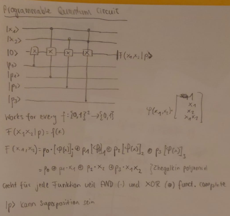
Boolean Fourier Transform

Every pseudo-boolean function can be represented as a polynomial in the form of a sum of products of boolean variables: f(x)=S[n]ωSiSxif(x) = \sum_{S \subseteq [n]} \omega _S \prod_{i \in S} x_i =S[n]ωSφS(x) = \sum_{S \subseteq [n]} \omega _S \varphi_S(x) =ωTφS(x) = \omega^T \varphi_S(x)

Example:

φ([x1,x2,x3])=[1x1x2x3x1x2x1x3x2x3x1x2x3]\varphi([x_1, x_2, x_3]) = \begin{bmatrix} 1 \\ x_1 \\ x_2 \\ x_3 \\ x_1 x_2 \\ x_1 x_3 \\ x_2 x_3 \\ x_1 x_2 x_3 \\ \end{bmatrix}

TODO task 1.6

Hadamard

Hadamard Matrix Definition

  • Hadamard Matrix: H1=12[1111]H_1 = \frac{1}{\sqrt{2}}\begin{bmatrix}1 & 1 \\ 1 & -1\end{bmatrix}
  • H0=[1]H_0 = [1]
  • For higher dimensions: Hn=H2Hn1H_n = H_2 \otimes H_{n-1}
  • H2=12[1111111111111111]H_2 = \frac{1}{2}\begin{bmatrix}1 & 1 & 1 & 1 \\ 1 & -1 & 1 & -1 \\ 1 & 1 & -1 & -1 \\ 1 & -1 & -1 & 1\end{bmatrix}

Hadamard Transform

Because the Hadamard matrix is unitary, it is involutory. If we want to solve f=Hnwf = H_n \cdot w for ww, we can calculate it directly: w=Hnfw = H_n \cdot f

Fourier

Fourier Matrix Definition

  • Fourier Matrix: Fn=12n[11111ωω2ω31ω2ω4ω61ω3ω6ω9]F_n = \frac{1}{\sqrt{2^n}}\begin{bmatrix}1 & 1 & 1 & 1 & \cdots \\ 1 & \omega & \omega^2 & \omega^3 & \cdots \\ 1 & \omega^2 & \omega^4 & \omega^6 & \cdots \\ 1 & \omega^3 & \omega^6 & \omega^9 & \cdots \\ \vdots & \vdots & \vdots & \vdots & \ddots\end{bmatrix}
  • ω=exp2πi2n\omega = \exp{\frac{2\pi i}{2^n}}
  • ω\omega is a primitive 2n2^n-th root of unity

Fourier Transform

Because the Fourier matrix is unitary, it is involutory. If we want to solve f=Fnwf = F_n \cdot w for ww, we can calculate it directly: w=Fnfw = F_n \cdot f

TODO task 2.3 b)

Bool-Möbius Transform

Sierpinski Matrix

  • Sierpinski Matrix:
    • S1=[1011]S_1 = \begin{bmatrix}1 & 0 \\ 1 & 1\end{bmatrix}
    • Sn=S1Sn1S_n = S_1 \otimes S_{n-1}
    • S2=[1000110010101111]S_2 = \begin{bmatrix}1 & 0 & 0 & 0 \\ 1 & 1 & 0 & 0 \\ 1 & 0 & 1 & 0 \\ 1 & 1 & 1 & 1\end{bmatrix}

Bool-Möbius Transform

Because Sn×Sn=IS_n\times S_n = I, the Sierpinski matrix is involutory. If we want to solve f=Snwf = S_n \cdot w for ww, we can calculate it directly: w=Snfw = S_n \cdot f

Yet another Feature Transform

Compared to our original

φ([x1,x2,x3])=[1x1x2x3x1x2x1x3x2x3x1x2x3]\varphi([x_1, x_2, x_3]) = \begin{bmatrix} 1 \\ x_1 \\ x_2 \\ x_3 \\ x_1 x_2 \\ x_1 x_3 \\ x_2 x_3 \\ x_1 x_2 x_3 \\ \end{bmatrix}

we now have

ϕ([x1,x2,x3])=[1x1x2x1x2x3x1x3x2x3x1x2x3]\phi([x_1, x_2, x_3]) = \begin{bmatrix} 1 \\ x_1 \\ x_2 \\ x_1 x_2 \\ x_3 \\ x_1 x_3 \\ x_2 x_3 \\ x_1 x_2 x_3 \\ \end{bmatrix}

Recursive definition: ϕ([])=[1]\phi([]) = [1] ϕ([x1,x2,,xn])=[1xn]ϕ([x1,x2,,xn1])\phi([x_1, x_2, \ldots, x_n]) = \begin{bmatrix} 1 \\ x_n \end{bmatrix} \otimes \phi([x_1, x_2, \ldots, x_{n-1}])

Pauli Matrices

  • The Pauli Matrices are unitary and involutory.
  • They can easily be written as linear combinations of outer products:
  • I=00+11=(1001)I = |0\rangle\langle0| + |1\rangle\langle1| = \begin{pmatrix}1 & 0 \\ 0 & 1\end{pmatrix}
  • X=01+10=(0110)X = |0\rangle\langle1| + |1\rangle\langle0| = \begin{pmatrix}0 & 1 \\ 1 & 0\end{pmatrix}
  • Y=i01+i10=(0ii0)Y = -i|0\rangle\langle1| + i|1\rangle\langle0| = \begin{pmatrix}0 & -i \\ i & 0\end{pmatrix}
  • Z=0011=(1001)Z = |0\rangle\langle0| - |1\rangle\langle1| = \begin{pmatrix}1 & 0 \\ 0 & -1\end{pmatrix}
  • Because they are unitary, their Eigenvalues are of norm 1. Because they are Hermitian, their Eigenvalues are real. Therefore, the Eigenvalues of the Pauli Matrices are ±1\pm 1.
  • Because they are Hermitian, their Eigenvectors are orthogonal.
  • Their Eigenvectors are:
    • II: (10)\begin{pmatrix}1 \\ 0\end{pmatrix} and (01)\begin{pmatrix}0 \\ 1\end{pmatrix}
    • XX: (11)\begin{pmatrix}1 \\ 1\end{pmatrix} and (11)\begin{pmatrix}1 \\ -1\end{pmatrix}
    • ZZ: (10)\begin{pmatrix}1 \\ 0\end{pmatrix} and (01)\begin{pmatrix}0 \\ 1\end{pmatrix}
    • YY: (1i)\begin{pmatrix}1 \\ i\end{pmatrix} and (1i)\begin{pmatrix}1 \\ -i\end{pmatrix}

Matrix Exponential

eiθX=cos(θ)I+isin(θ)Xe^{i\theta X} = \cos(\theta)I + i\sin(\theta)X

Therefore,

  • RX(θ)=eiθX=cos(θ)Iisin(θ)XR_X(\theta) = e^{-i\theta X} = \cos(\theta)I - i\sin(\theta)X
  • RY(θ)=eiθY=cos(θ)Iisin(θ)YR_Y(\theta) = e^{-i\theta Y} = \cos(\theta)I - i\sin(\theta)Y
  • RZ(θ)=eiθZ=cos(θ)Iisin(θ)ZR_Z(\theta) = e^{-i\theta Z} = \cos(\theta)I - i\sin(\theta)Z

Linear Combinations of Pauli Matrices

Every matrix AC2×2A \in \mathbb{C}^{2\times 2} can be written as a linear combination of the Pauli Matrices.

This is because we can write the standard basis as a linear combination of the Pauli Matrices:

00=12(I+Z)|0\rangle \langle 0| = \frac{1}{2}(I + Z) 11=12(IZ)|1\rangle \langle 1| = \frac{1}{2}(I - Z) 01=12(X+iY)|0\rangle \langle 1| = \frac{1}{2}(X + iY) 10=12(XiY)|1\rangle \langle 0| = \frac{1}{2}(X - iY)

A=12(Tr(A)I+Tr(AX)X+Tr(AY)Y+Tr(AZ)Z)A = \frac{1}{2}\left(\text{Tr}(A)I + \text{Tr}(AX)X + \text{Tr}(AY)Y + \text{Tr}(AZ)Z\right)

Example

The Matrix V=12[ii11]V = \frac{1}{\sqrt{2}} \begin{bmatrix} i & -i \\ 1 & 1 \end{bmatrix}

Beam Splitter

B=12[1ii1]B=\frac{1}{\sqrt{2}}\begin{bmatrix}1 & i \\ i & 1\end{bmatrix}

Wiederholt sich beim Quadrieren.

Bivariate Functions as 2x2 Matrices

Every bivariate function can be represented as a 2x2 matrix.

With x=[1x]x=\begin{bmatrix}1\\x\end{bmatrix} and y=[1y]y=\begin{bmatrix}1\\y\end{bmatrix}, we can write the function ff as

xT[abcd]y=a+by+cx+dxyx^T \begin{bmatrix}a & b \\ c & d\end{bmatrix} y = a + by + cx + dxy

x y Expression for xT M y
0 0 a
1 0 a + c
0 1 a + b
1 1 a + b + c + d
Coefficient Expression
a f(0,0)
b f(0,1) - a
c f(1,0) - a
d f(1,1) - a - b - c

3D Vectors as Matrices

Every 3D vector can be represented as a matrix.

X((x1x2x3))=[x3x1ix2x1+ix2x3]X(\begin{pmatrix}x_1\\x_2\\x_3\end{pmatrix}) = \begin{bmatrix} x_3 & x_1 - ix_2 \\ x_1 + ix_2 & -x_3 \end{bmatrix}

X((100))=[0110]=XX(\begin{pmatrix}1\\0\\0\end{pmatrix}) = \begin{bmatrix} 0 & 1 \\ 1 & 0 \end{bmatrix} = X X((010))=[0ii0]=YX(\begin{pmatrix}0\\1\\0\end{pmatrix}) = \begin{bmatrix} 0 & -i \\ i & 0 \end{bmatrix} = Y X((001))=[1001]=ZX(\begin{pmatrix}0\\0\\1\end{pmatrix}) = \begin{bmatrix} 1 & 0 \\ 0 & -1 \end{bmatrix} = Z

Note the following:

xTy=12Tr(XY)x^Ty = \frac{1}{2}\text{Tr}(XY)

And for square matrices: Tr(AB)=Tr(BA)\text{Tr}(AB) = \text{Tr}(BA)

Therefore, the inner product of 2 real vectors is symmetric

Born Rule

the spatial component of the wave function of a 1D particle trapped in a 1D well is given by

ψn(x)=2wsin(nπxw)\psi_n(x) = \sqrt{\frac{2}{w}} \sin\left(\frac{n \pi x}{w}\right)

for 0xw and by\text{for } 0 \leq x \leq w \text{ and by}

ψn(x)=0\psi_n(x) = 0

elsewhere.

Hamiltonian is Hermitianeigenvectors are orthogonal\text{Hamiltonian is Hermitian} \Rightarrow \text{eigenvectors are orthogonal}

Inner Product is 0 when orthogonal, i.e., when two different eigenvectors are multiplied, the result is 0.

If we have two identical eigenvectors:

ψnψn=0w2wsin2(nπxw)dx=201sin2(nπx)dx\int \psi_n^* \psi_n = \int_0^w \frac{2}{w} \sin^2\left(\frac{n \pi x}{w}\right) dx = 2 \int_0^1 \sin^2\left(n \pi x\right) dx =2nπ0nπsin2(x)dx=1= \frac{2}{n\pi} \int_0^{n\pi} \sin^2(x) dx = 1

4th roots of unity

Gn={e2πik/nk{0,1,2,3}}G_n = \left\{ e^{2\pi i k / n} \mid k \in \{0, 1, 2, 3\} \right\}

Rotations in the complex plane

To rotate a complex number by an angle, we multiply it by ix=ex×ln(i)i^x = e^{x\times\ln(i)}

What is ln(i)\ln(i)?

eix=isin(x)+cos(x)e^{ix} = i\,\sin(x) + \cos(x)

eln(i)=ieln(i)i=ie^{\ln(i)} = i \quad\Longrightarrow\quad e^{\frac{\ln(i)}{i}} = i

i=isin ⁣(ln(i)i)+cos ⁣(ln(i)i)\Longrightarrow\quad i = i\,\sin\!\Bigl(\frac{\ln(i)}{i}\Bigr) + \cos\!\Bigl(\frac{\ln(i)}{i}\Bigr) ln(i)i=π2ln(i)=iπ2\Longrightarrow\quad \frac{\ln(i)}{i} = \frac{\pi}{2} \quad\Longrightarrow\quad \ln(i) = i\,\frac{\pi}{2}

Phase Gate

S=[100i]S = \begin{bmatrix} 1 & 0 \\ 0 & i \end{bmatrix}

It is the generator of:

G={[100ei2π/n]kkZ} G= \{\begin{bmatrix} 1 & 0 \\ 0 & e^{i2\pi /n} \end{bmatrix}^k | k \in \Z \}

Quaternions

Quaternions are a non-commutative extension of complex numbers.

i2=j2=k2=ijk=1i^2 = j^2 = k^2 = ijk = -1 ij=k,jk=i,ki=jij = k, jk = i, ki = j ji=k,kj=i,ik=jji = -k, kj = -i, ik = -j

Quaternions as Matrices

The matrices for (i), (j), and (k) are given as:

i=[0100100000010010]i = \begin{bmatrix} 0 & -1 & 0 & 0 \\ 1 & 0 & 0 & 0 \\ 0 & 0 & 0 & -1 \\ 0 & 0 & 1 & 0 \end{bmatrix} j=[0001001001001000]j = \begin{bmatrix} 0 & 0 & 0 & -1 \\ 0 & 0 & 1 & 0 \\ 0 & -1 & 0 & 0 \\ 1 & 0 & 0 & 0 \end{bmatrix} k=[0010000110000100]k = \begin{bmatrix} 0 & 0 & -1 & 0 \\ 0 & 0 & 0 & -1 \\ 1 & 0 & 0 & 0 \\ 0 & 1 & 0 & 0 \end{bmatrix}

The product (ijk) gives:

ij=[0010000110000100]=ki \cdot j = \begin{bmatrix} 0 & 0 & -1 & 0 \\ 0 & 0 & 0 & -1 \\ 1 & 0 & 0 & 0 \\ 0 & 1 & 0 & 0 \end{bmatrix} = k

Finally, multiplying further:

ijk=Ii \cdot j \cdot k = -I

This aligns with (ijk = -1).

TODO 4.9

Vector Logic

Example

Given a matrix

C=n[nn]T+n[ns]T+n[sn]T+s[ss]TC = n[n\otimes n]^T + n[n\otimes s]^T + n[s \otimes n]^T + s[s \otimes s]^T =[11100001] = \begin{bmatrix} 1 & 1&1&0 \\ 0&0&0&1 \end{bmatrix}

multiplying it with, say, [1000]\begin{bmatrix} 1 \\ 0 \\ 0 \\ 0 \end{bmatrix} gives you the first column of the matrix, which is [10]\begin{bmatrix} 1 \\ 0 \end{bmatrix}.

You can also write C as:

C=FnT+IsTC = F \otimes n^T + I \otimes s^T

because the kronecker product is linear.

Bilinearity of the Kronecker Product

We start with:

xy=(j=1mxjuj)(k=1nykvk).|x\rangle \otimes |y\rangle = \left(\sum_{j=1}^m x_j \, |u_j\rangle\right) \otimes \left(\sum_{k=1}^n y_k \, |v_k\rangle\right).

Distributing the terms:

=j=1mk=1n(xjuj)(ykvk).= \sum_{j=1}^m \sum_{k=1}^n \bigl(x_j \, |u_j\rangle\bigr) \otimes \bigl(y_k \, |v_k\rangle\bigr).

Which simplifies to:

=j=1mk=1nxjyk(ujvk).= \sum_{j=1}^m \sum_{k=1}^n x_j \, y_k \bigl(|u_j\rangle \otimes |v_k\rangle\bigr).

Tensor Products and the Born Rule

If we have two states a|a\rangle and b|b\rangle that obey the Born rule, then the tensor product of these states also obeys the Born rule.

Comments

Feel free to leave your opinion or questions in the comment section below.